Getting started

The easiest way to get started with GeoProfile is in the Jupyter Notebook.

Installation

To install this package, including the map and gef reading functionality, run:

pip install geoprofile[map, gef]

To skip the installation of the GeoProfile library, in case you do not need it (e.g. only use pure plotting), run:

pip install geoprofile

Than you can import proficore as follows:

In [1]: from geoprofile.column import Column

In [2]: from geoprofile.profile import Section

In [3]: import numpy as np

In [4]: import plotly.io as pio

In [5]: from shapely.geometry import LineString

or any equivalent import statement.

Create Columns

The first thing to do is to create column classes. This class holds the information of the for example a CPT or borehole. For more information on the geoprofile.column.Column() class go the the reference.

In [6]: columns = [
   ...:     Column(
   ...:         classify={
   ...:             "depth": [5, -10, -20, -30],
   ...:             "thickness": [15, 10, 10, 10],
   ...:             "geotechnicalSoilName": [
   ...:                 "sterkGrindigZand",
   ...:                 "zwakZandigSiltMetGrind",
   ...:                 "sterkZandigeDetritus",
   ...:                 "grind",
   ...:             ],
   ...:         },
   ...:         x=0,
   ...:         y=0,
   ...:         z=-1,
   ...:         name="A",
   ...:     ),
   ...:     Column(
   ...:         classify={
   ...:             "depth": [0, -10, -20, -30],
   ...:             "thickness": [10, 10, 10, 10],
   ...:             "geotechnicalSoilName": [
   ...:                 "sterkGrindigZand",
   ...:                 "zwakZandigSiltMetGrind",
   ...:                 "sterkZandigeDetritus",
   ...:                 "grind",
   ...:             ],
   ...:         },
   ...:         x=-3,
   ...:         y=50,
   ...:         z=4,
   ...:         name="B",
   ...:         data={
   ...:             "depth": np.linspace(0, -40).tolist(),
   ...:             "qc": np.random.random(50).tolist(),
   ...:             "abc": np.random.random(50).tolist(),
   ...:         },
   ...:     ),
   ...:     Column(
   ...:         classify={
   ...:             "depth": [0, -10, -20, -30],
   ...:             "thickness": [10, 10, 10, 10],
   ...:             "geotechnicalSoilName": [
   ...:                 "sterkGrindigZand",
   ...:                 "zwakZandigSiltMetGrind",
   ...:                 "sterkZandigeDetritus",
   ...:                 "grind",
   ...:             ],
   ...:         },
   ...:         x=4,
   ...:         y=10,
   ...:         z=3,
   ...:         name="C",
   ...:         data={
   ...:             "depth": np.linspace(0, -40).tolist(),
   ...:             "qc": np.random.random(50).tolist(),
   ...:             "abc": np.random.random(50).tolist(),
   ...:         },
   ...:     ),
   ...:     Column(
   ...:         classify={
   ...:             "depth": [0, -10, -20, -30],
   ...:             "thickness": [10, 10, 10, 10],
   ...:             "geotechnicalSoilName": [
   ...:                 "sterkGrindigZand",
   ...:                 "zwakZandigSiltMetGrind",
   ...:                 "sterkZandigeDetritus",
   ...:                 "grind",
   ...:             ],
   ...:         },
   ...:         x=-30,
   ...:         y=30,
   ...:         z=-5,
   ...:         name="D",
   ...:         data={
   ...:             "depth": np.linspace(0, -40).tolist(),
   ...:             "qc": np.random.random(50).tolist(),
   ...:             "abc": np.random.random(50).tolist(),
   ...:         },
   ...:     ),
   ...:     Column(
   ...:         classify={
   ...:             "depth": [0, -10, -20, -30],
   ...:             "thickness": [10, 10, 10, 10],
   ...:             "geotechnicalSoilName": [
   ...:                 "sterkGrindigZand",
   ...:                 "zwakZandigSiltMetGrind",
   ...:                 "sterkZandigeDetritus",
   ...:                 "grind",
   ...:             ],
   ...:         },
   ...:         x=-5,
   ...:         y=30,
   ...:         z=1,
   ...:         name="E",
   ...:         data={
   ...:             "depth": np.linspace(0, -40).tolist(),
   ...:             "qc": np.random.random(50).tolist(),
   ...:             "abc": np.random.random(50).tolist(),
   ...:         },
   ...:     ),
   ...: ]
   ...: 

To plot the column as a standalone you can call the plot method of the class. Be default only the data in the classify dictionary is shown. To include data from the data dictionary use the plot_kwargs argument.

In [7]: fig = columns[1].plot(
   ...:     plot_kwargs={"qc": {"line_color":"black"}, "abc": {"line_color": "red"}}
   ...: )
   ...: 

Create Profile

The next step is to create a Section class. This class holds the information of all Columns. For more information on the geoprofile.column.Section() class go the the reference.

In [8]: profile = Section(
   ...:     columns,
   ...:     profile_line=LineString(((-1, 0), (3, 30), (1, 51))),
   ...:     sorting_algorithm="tsp",
   ...:     reproject=True,
   ...: )
   ...: 

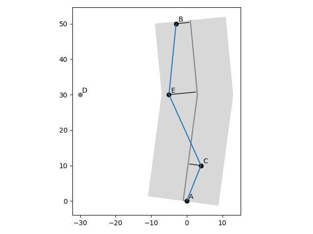
Different sorting algorithms can be used to sort the list of columns to the profile line. It is also possible to project the location of the column onto the profile line. To have an overview of al the column location, profile line and the section use the map plot.

In [9]: profile.plot_map()
Out[9]: <Axes: >

If you happy with your profile line you can plot the section as follows:

In [10]: fig = profile.plot(
   ....:     plot_kwargs={"qc": {}, "abc": {}},
   ....:     hue="uniform",
   ....:     fillpattern=False,
   ....:     surface_level=True,
   ....:     groundwater_level=True,
   ....: )
   ....: