Installing pygef
To install pygef, we strongly recommend using Python Package Index (PyPI).
You can install pygef with:
pip install pygef[map,plot]
We installed the map variant of pygef which include additional dependencies,
and thereby enable additional functionality.
How to import pygef
Getting started with pygef is easy done by importing the pygef library:
In [1]: import pygef

In [2]: from pygef.plotting import plot_bore, plot_cpt, plot_merge
or any equivalent import statement.
Load a Cpt/Bore file
The classes read_cpt and read_bore accept two possible inputs:
the
pathof the filethe
BytesIOof the file
If you want to use the path then your code should look like this:
In [3]: import os

In [4]: path_cpt = os.path.join(
   ...:     os.environ.get("DOC_PATH"), "../tests/test_files/cpt_xml/example.xml"
   ...: )
   ...:

In [5]: cpt = pygef.read_cpt(path_cpt)
Access the attributes
Accessing the attributes of a pygef object is quite easy. If for example we want to know the (x, y, z) coordinates of the gef we can simply do:
In [6]: coordinates = (
   ...:     cpt.standardized_location.x,
   ...:     cpt.standardized_location.y,
   ...:     cpt.delivered_vertical_position_offset
   ...: )
   ...:

In [7]: print(coordinates)
(52.36533659, 5.60907955, 4.41)
Check all the available attributes in the reference. Everything (or almost) that is contained in the files it is now
accessible as attribute of the gef object.
The classes pygef.cpt.CPTData() and pygef.bore.BoreData() have different attributes, check the reference to learn more about it.
A common and very useful attribute is CPTData.data, this is a polars.DataFrame that contains all the rows and
columns defined in the file.
CPT
If we call CPTData.data on a CPTData object we will get something like this:
In [8]: cpt.data
Out[8]:
shape: (372, 11)
┌────────────┬───────┬────────────┬────────────┬───┬───────────┬───────────┬───────────┬───────────┐
│ penetratio ┆ depth ┆ elapsedTim ┆ coneResist ┆ … ┆ localFric ┆ frictionR ┆ depthOffs ┆ frictionR │
│ nLength    ┆ ---   ┆ e          ┆ ance       ┆   ┆ tion      ┆ atio      ┆ et        ┆ atioCompu │
│ ---        ┆ f64   ┆ ---        ┆ ---        ┆   ┆ ---       ┆ ---       ┆ ---       ┆ ted       │
│ f64        ┆       ┆ f64        ┆ f64        ┆   ┆ f64       ┆ f64       ┆ f64       ┆ ---       │
│            ┆       ┆            ┆            ┆   ┆           ┆           ┆           ┆ f64       │
╞════════════╪═══════╪════════════╪════════════╪═══╪═══════════╪═══════════╪═══════════╪═══════════╡
│ 0.02       ┆ 0.02  ┆ 11.0       ┆ 2.708      ┆ … ┆ 0.03      ┆ 0.6       ┆ 4.39      ┆ 1.107829  │
│ 0.04       ┆ 0.039 ┆ 13.0       ┆ 4.29       ┆ … ┆ 0.039     ┆ 0.8       ┆ 4.371     ┆ 0.909091  │
│ 0.06       ┆ 0.059 ┆ 15.0       ┆ 5.124      ┆ … ┆ 0.045     ┆ 0.9       ┆ 4.351     ┆ 0.87822   │
│ 0.08       ┆ 0.079 ┆ 17.0       ┆ 5.45       ┆ … ┆ 0.049     ┆ 1.0       ┆ 4.331     ┆ 0.899083  │
│ 0.1        ┆ 0.099 ┆ 19.0       ┆ 5.41       ┆ … ┆ 0.056     ┆ 1.0       ┆ 4.311     ┆ 1.03512   │
│ …          ┆ …     ┆ …          ┆ …          ┆ … ┆ …         ┆ …         ┆ …         ┆ …         │
│ 7.36       ┆ 7.359 ┆ 519.0      ┆ 10.815     ┆ … ┆ null      ┆ 0.0       ┆ -2.949    ┆ null      │
│ 7.38       ┆ 7.379 ┆ 520.0      ┆ 10.576     ┆ … ┆ null      ┆ 0.0       ┆ -2.969    ┆ null      │
│ 7.4        ┆ 7.399 ┆ 521.0      ┆ 10.235     ┆ … ┆ null      ┆ 0.0       ┆ -2.989    ┆ null      │
│ 7.42       ┆ 7.419 ┆ 522.0      ┆ 9.714      ┆ … ┆ null      ┆ 0.0       ┆ -3.009    ┆ null      │
│ 7.44       ┆ 7.439 ┆ 523.0      ┆ 9.11       ┆ … ┆ null      ┆ 0.0       ┆ -3.029    ┆ null      │
└────────────┴───────┴────────────┴────────────┴───┴───────────┴───────────┴───────────┴───────────┘
The number and type of columns depends on the columns originally present in the cpt.
The columns penetration_length, qc, depth are always present.
Suggestion: Instead of using the column penetration_length use the column depth since this one is corrected with the inclination (if present).
Borehole
If we call BoreData.data on a BoreData object we will get something like this:
In [9]: path_bore = os.path.join(
   ...:     os.environ.get("DOC_PATH"), "../tests/test_files/bore_xml/DP14+074_MB_KR.xml"
   ...: )
   ...:

In [10]: bore = pygef.read_bore(path_bore)

In [11]: bore.data
Out[11]:
shape: (13, 10)
┌───────────┬───────────┬───────────┬───────────┬───┬───────────┬───────────┬───────────┬──────────┐
│ upperBoun ┆ lowerBoun ┆ geotechni ┆ color     ┆ … ┆ sandMedia ┆ upperBoun ┆ lowerBoun ┆ soilDist │
│ dary      ┆ dary      ┆ calSoilNa ┆ ---       ┆   ┆ nClass    ┆ daryOffse ┆ daryOffse ┆ ribution │
│ ---       ┆ ---       ┆ me        ┆ str       ┆   ┆ ---       ┆ t         ┆ t         ┆ ---      │
│ f64       ┆ f64       ┆ ---       ┆           ┆   ┆ str       ┆ ---       ┆ ---       ┆ list[f64 │
│           ┆           ┆ str       ┆           ┆   ┆           ┆ f64       ┆ f64       ┆ ]        │
╞═══════════╪═══════════╪═══════════╪═══════════╪═══╪═══════════╪═══════════╪═══════════╪══════════╡
│ 0.0       ┆ 1.0       ┆ zwakGrind ┆ donkergri ┆ … ┆ middelgro ┆ 10.773    ┆ 9.773     ┆ [0.0,    │
│           ┆           ┆ igZand    ┆ js        ┆   ┆ f420tot63 ┆           ┆           ┆ 0.2, …   │
│           ┆           ┆           ┆           ┆   ┆ 0um       ┆           ┆           ┆ 0.0]     │
│ 1.0       ┆ 1.1       ┆ zwakGrind ┆ donkergri ┆ … ┆ middelgro ┆ 9.773     ┆ 9.673     ┆ [0.0,    │
│           ┆           ┆ igZand    ┆ js        ┆   ┆ f420tot63 ┆           ┆           ┆ 0.2, …   │
│           ┆           ┆           ┆           ┆   ┆ 0um       ┆           ┆           ┆ 0.0]     │
│ 1.1       ┆ 2.0       ┆ zwakZandi ┆ standaard ┆ … ┆ null      ┆ 9.673     ┆ 8.773     ┆ [0.0,    │
│           ┆           ┆ geKleiMet ┆ Bruin     ┆   ┆           ┆           ┆           ┆ 0.1, …   │
│           ┆           ┆ Grind     ┆           ┆   ┆           ┆           ┆           ┆ 0.0]     │
│ 2.0       ┆ 3.0       ┆ zwakZandi ┆ standaard ┆ … ┆ null      ┆ 8.773     ┆ 7.773     ┆ [0.0,    │
│           ┆           ┆ geKlei    ┆ Grijs     ┆   ┆           ┆           ┆           ┆ 0.0, …   │
│           ┆           ┆           ┆           ┆   ┆           ┆           ┆           ┆ 0.0]     │
│ 3.0       ┆ 4.0       ┆ zwakZandi ┆ donkergri ┆ … ┆ null      ┆ 7.773     ┆ 6.773     ┆ [0.0,    │
│           ┆           ┆ geKlei    ┆ js        ┆   ┆           ┆           ┆           ┆ 0.0, …   │
│           ┆           ┆           ┆           ┆   ┆           ┆           ┆           ┆ 0.0]     │
│ …         ┆ …         ┆ …         ┆ …         ┆ … ┆ …         ┆ …         ┆ …         ┆ …        │
│ 7.0       ┆ 8.0       ┆ siltigZan ┆ lichtgrij ┆ … ┆ fijn150to ┆ 3.773     ┆ 2.773     ┆ [0.0,    │
│           ┆           ┆ d         ┆ s         ┆   ┆ t200um    ┆           ┆           ┆ 0.0, …   │
│           ┆           ┆           ┆           ┆   ┆           ┆           ┆           ┆ 0.0]     │
│ 8.0       ┆ 9.0       ┆ siltigZan ┆ standaard ┆ … ┆ fijn150to ┆ 2.773     ┆ 1.773     ┆ [0.0,    │
│           ┆           ┆ d         ┆ Grijs     ┆   ┆ t200um    ┆           ┆           ┆ 0.0, …   │
│           ┆           ┆           ┆           ┆   ┆           ┆           ┆           ┆ 0.0]     │
│ 9.0       ┆ 10.0      ┆ siltigZan ┆ standaard ┆ … ┆ fijn150to ┆ 1.773     ┆ 0.773     ┆ [0.0,    │
│           ┆           ┆ d         ┆ Grijs     ┆   ┆ t200um    ┆           ┆           ┆ 0.0, …   │
│           ┆           ┆           ┆           ┆   ┆           ┆           ┆           ┆ 0.0]     │
│ 10.0      ┆ 11.0      ┆ siltigZan ┆ standaard ┆ … ┆ middelgro ┆ 0.773     ┆ -0.227    ┆ [0.0,    │
│           ┆           ┆ dMetGrind ┆ Grijs     ┆   ┆ f200tot30 ┆           ┆           ┆ 0.15, …  │
│           ┆           ┆           ┆           ┆   ┆ 0um       ┆           ┆           ┆ 0.0]     │
│ 11.0      ┆ 12.0      ┆ siltigZan ┆ standaard ┆ … ┆ middelgro ┆ -0.227    ┆ -1.227    ┆ [0.0,    │
│           ┆           ┆ dMetGrind ┆ Grijs     ┆   ┆ f300tot42 ┆           ┆           ┆ 0.15, …  │
│           ┆           ┆           ┆           ┆   ┆ 0um       ┆           ┆           ┆ 0.0]     │
└───────────┴───────────┴───────────┴───────────┴───┴───────────┴───────────┴───────────┴──────────┘
Plot a gef file
We can plot a gef file using the method .plot(), check the reference to know which are the arguments of the method.
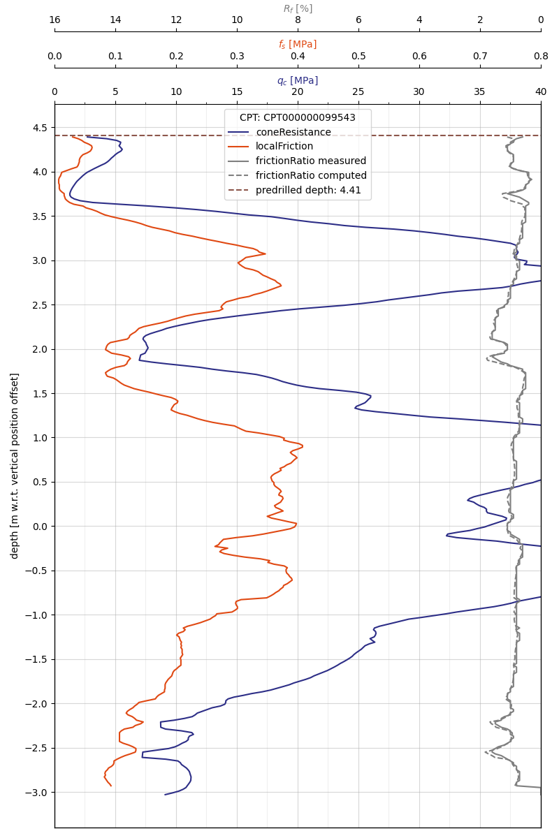
CPT
If we use the method without arguments on a cpt object we get:
In [12]: pygef.plotting.plot_cpt(cpt, use_offset=True)
Out[12]:
(<Axes: xlabel='$q_c$ [MPa]', ylabel='depth [m w.r.t. vertical position offset]'>,
 <Axes: xlabel='$f_s$ [MPa]'>,
 <Axes: xlabel='$R_f$ [%]'>)
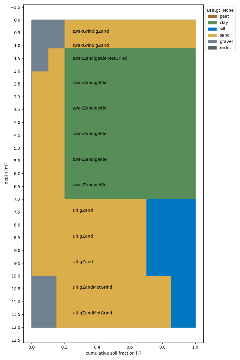
Borehole
If we use the method without arguments on a BoreData object we get:
In [13]: pygef.plotting.plot_bore(bore)
Out[13]: <Axes: xlabel='cumulative soil fraction [-]', ylabel='depth [m]'>
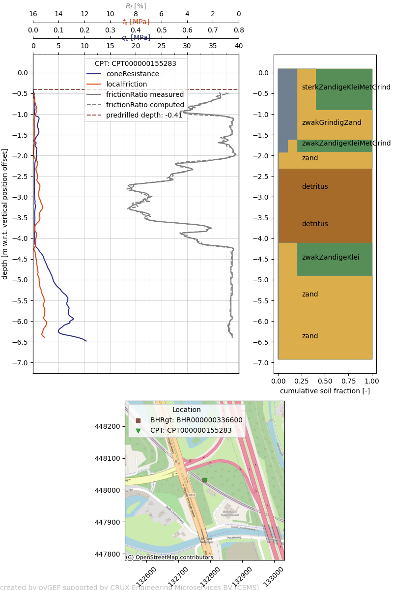
Combine Borehole an CPT
# parse BRO bhrgt XML
In [14]: path_bore = os.path.join(
   ....:     os.environ.get("DOC_PATH"), "../tests/test_files/bore_xml/BHR000000336600.xml"
   ....: )
   ....:

In [15]: bore = pygef.read_bore(path_bore)

# parse BRO CPT XML
In [16]: path_cpt = os.path.join(
   ....:     os.environ.get("DOC_PATH"), "../tests/test_files/cpt_xml/CPT000000155283.xml"
   ....: )
   ....:

In [17]: cpt = pygef.read_cpt(path_cpt)

In [18]: pygef.plotting.plot_merge(bore, cpt)
Out[18]:
(<Figure size 800x1200 with 5 Axes>,
 [<Axes: xlabel='$q_c$ [MPa]', ylabel='depth [m w.r.t. vertical position offset]'>,
  <Axes: xlabel='cumulative soil fraction [-]'>,
  <Axes: >])